LAB2 : Forward and Inverse Kinematics for the KUKA Robotic Arm Solution

Starting from:

$30

Home

1 Purpose

The purpose of this lab is to adapt the results of lab 1 for implementation in a real robot. The objective is to make the robot arm draw on paper.

2 Introduction

The KUKA robotic arm depicted in Figure 1 is an articulated manipulator with a three-degree-of-freedom wrist and a gripper. Highlighted in Figure 1 are the axes of rotation of joints 1 to 6. A pencil, not displayed

Figure 1: The KUKA robotic arm in the HOME configuration

in Figure 1, will be attached to the gripper and will point along the pencil heading direction indicated in the figure. The tip of the pencil is the end eﬀector of the robot. The objective of this lab is to make the robot draw patterns on paper.

The kinematic parameters of the robot are detailed in Figure 2. The red elements in the figure are the joint axes. The values of various parameters are found in the table below.

3 Preparation

Please submit a complete preparation at the beginning of the lab session. Prior to the lab, you should make sure that step 4 of the preparation returns consistent results. An incomplete or incorrect preparation will be penalized.

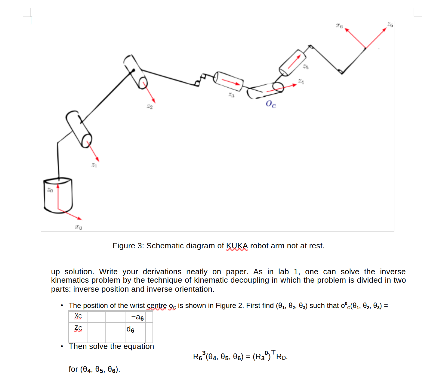
Figure 3 depicts the robot in a generic configuration away from the rest position. Print out this page and draw on the figure coordinate frames o₁x₁y₁z₁, o₂x₂y₂z₂, o₃x₃y₃z₃, o₄x₄y₄z₄ and o₅x₅y₅z₅ according to the DH convention, and write the DH table of the robot. In particular, choose the x₁ axis parallel to the x₀ axis, x₁ = x₀ (this is done for convenience).

If your DH frame assignment is correct, you should find that when θ₁ = θ₂ = θ₃ = 0, link 2 is parallel to the ground, and link 3 is vertical, pointing downward. A schematic diagram of the KUKA robot arm in the HOME configuration is illustrated in Figure 4 which you should verify corresponds to (θ₁, θ₂, θ₃, θ₄, θ₅, θ₆) = (0, π/2, 0, 0, π/2, 0).

Derive the inverse kinematics of the robot. Specifically, given R₆⁰(θ₁, . . . , θ₆) = R_D and o⁰₆(θ₁, . . . , θ₆) = o⁰_D, find (θ₁, θ₂, θ₃, θ₄, θ₅, θ₆). You will find two solutions: elbow up and elbow down. Find the elbow

Modify your inverse kinematics function from lab 1 to incorporate the changes of this setup. Specifically, write Matlab functions mykuka.m, forward kuka.m, and inverse kuka.m as follows.

myrobot = mykuka(DH) defines the robot structure of the KUKA robot with the 6 × 4 DH table you found earlier.

H = forward kuka(q,myrobot) returns the homogeneous transformation matrix H of the end eﬀector, where q is the 6 × 1 vector of joint angles, and myrobot is the robot structure defined above.

q = inverse kuka(H,myrobot) returns the 6 × 1 vector of joint angles q = (θ₁, θ₂, θ₃, θ₄, θ₅, θ₆), where

H is the 4 × 4 homogeneous transformation matrix H =

Test your software: you should get

kuka=mykuka(DH);

forward_kuka([pi/5 pi/3 -pi/4 pi/4 pi/3 pi/4]’,kuka)

ans =

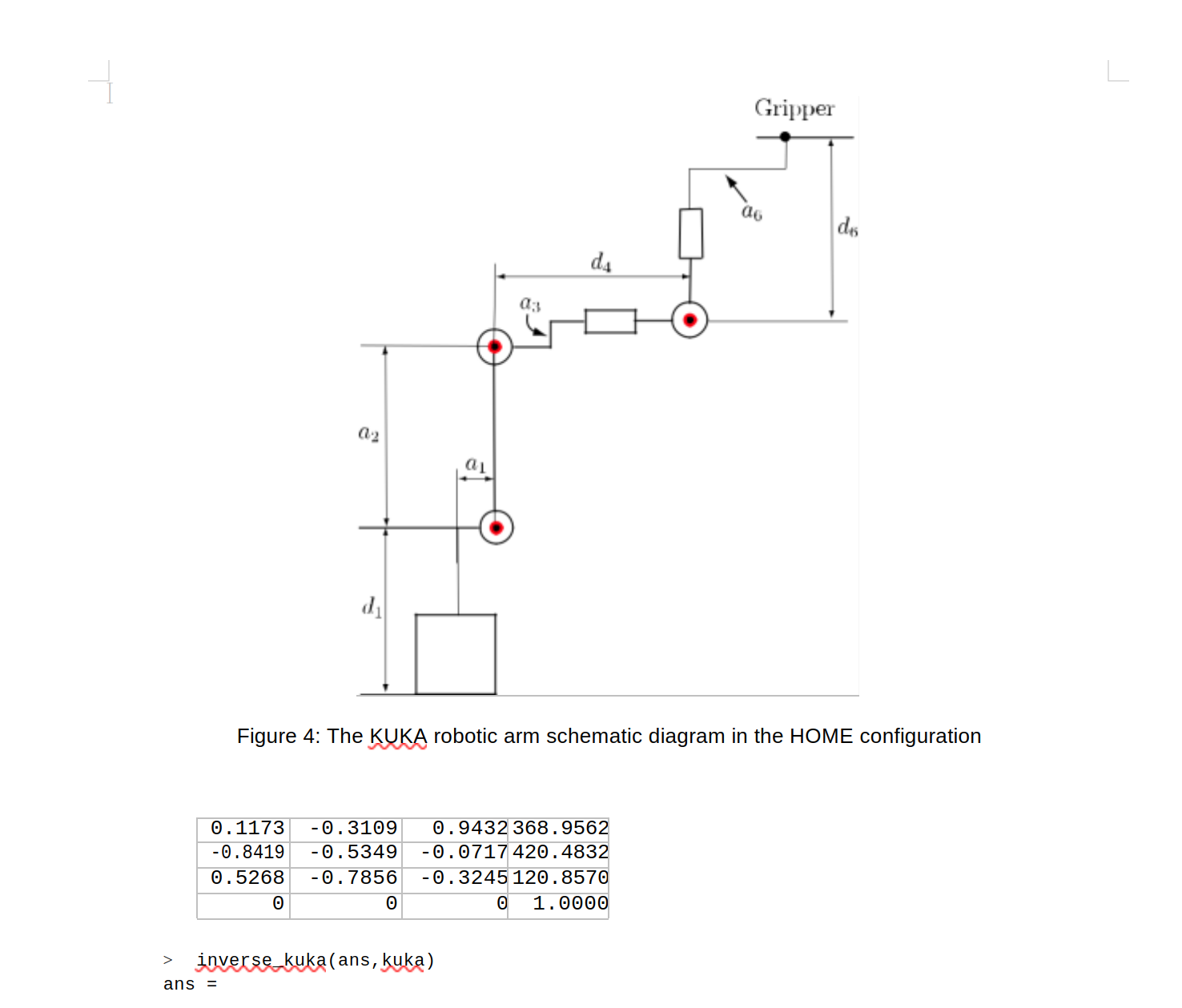
inverse_kuka(ans,kuka) ans =

0.6283

1.0472

-0.7854

0.7854

1.0472

0.7854

4 Experiment

In this lab you will learn to interface the KUKA robot with Matlab, you will then calibrate the DH parameters by taking measurements, and finally you will use the Matlab functions you developed in your preparation to make the robot draw patterns on paper. We begin by recalling the Matlab commands that you can use to control the Kuka robot arm.

4.1 Review: Commanding the KUKA robot arm through Matlab

For your reference, below are the Matlab commands you will use to control the Kuka robot arm. You have practiced these commands in Lab 0.

startConnection establishes connection between Matlab and KUKA.

stopConnection terminates connection between Matlab and KUKA.

getAngles() returns the vector of current joint angles q = (θ₁, θ₂, θ₃, θ₄, θ₅, θ₆).

stop() stops KUKA motion.

moveAxis(axis,vel) moves a single KUKA axis. axis takes a value between 1 and 6 that corresponds to the joint angle to be commanded. vel is a signed value that determines the commanded angular speed of the joint. In this lab vel should be set to no greater than 0.01.

setAngles(q,vel) sets KUKA arm angles to those defined in q to within a small tolerance. vel corresponds to the speed of motion. For this lab, set vel to 0.04. To cancel the command during execution press ctrl c and run stop() in the Matlab command window.

setHome(vel) sets KUKA arm to the HOME configuration in Figure 1. vel corresponds to the speed of motion. For this lab, set vel to 0.04. To cancel the command during execution press ctrl c and run stop() in the Matlab command window.

setGripper(state) sets the gripper state. setGripper(0) closes the gripper; setgripper(1) opens the gripper.

Warning: Never use the clear all command in Matlab. Instead use clearvars -except udpObj to avoid errors from occurring.

The steps to connect KUKA to the external PC:

Run startConnection in Matlab.

On the KUKA SmartPad run RSI Ethernet.src until the line RSI MOVECORR().

To run the program, hold down half-way one of the enable buttons on the back of the KUKA SmartPAD. The enable buttons are labelled 3 and 5 in Figure 5. If you press too hard, an emergency stop will be activated. While holding down the enable button, press and hold the run button labelled 10 in Figure 6. Note that when running the line RSI ON a warning will appear saying ‘Caution - sensor correction is activated”. Simply confirm this warning to continue.

The steps to command the KUKA arm from Matlab are as follows:

Run the desired command in the Matlab command window. The robot will not yet move.

Hold down half-way one of the enable buttons on the back of the KUKA SmartPAD.

While holding down the enable button, press and hold the run button. Now the robot will carry out the desired command as long as both the enable and run buttons are being held down.

To make the robot stop moving, simply release the enable button. To cancel the current command, press ctrl c and run stop().

Figure 5: 3 and 5 are Enable buttons on the KUKA SmartPAD.

If the robot ever hits an object while moving (such as the ground), immediately release the enable button and the robot will stop. Then press ctrl c in the Matlab control window to cancel the command and run stop(). Immediately call a TA to resolve the collision.

If the robot does not move when commanded, it means an error has occurred. Call a TA to resolve the issue.

For safety, students must never open the safety gate enclosing the robot unless instructed to do so. The enable and start button must never be pressed while the safety gate is open.

Warning: Make sure to FIRST connect KUKA to Matlab using startConnection.m. THEN run the RSI from the Kuka SmartPad

The steps to disconnect KUKA from the external PC:

When finished running the lab, return to the program RSI Ethernet.src on the SmartPAD, click on line 32 and then click Block selection to set the program cursor to the command ret=RSI OFF(). Then continue running the program to the end. The program status indicator will turn black to indicate the program is complete.

Run stopConnection in Matlab.

The steps to deal with an RSI connection problem:

Type CTRL+C within the Matlab environment.

There are two options available on the top portion of the SmartPAD screen: cancel or reset. Use reset, not cancel, to reinitialize the RSI program from the Kuka SmartPAD.

After resetting the RSI program, push the play button multiple times until the program reaches the

RSI MOVECORR() line.

Figure 6: 10 is the Run button on the KUKA SmartPAD.

In Matlab, run getAngles() to verify that the RSI connection has been correctly re-established.

4.2 Calibration of DH parameters

The DH parameters provided to you in the preparation were approximate. You need to calibrate them in order to improve the accuracy of the forward kinematics function. The main source of the inaccuracy are the parameters a₆, and d₆. We will tune these using a simple optimization approach. These are the steps we will perform to calibrate the robot:

Data collection. We will collect data pairs (Q_I, X_I) for three sample points, where Q_I is the joint vector of the robot, and X_I is the corresponding position of the pencil tip in frame 0.

Parametric robot structure. We will parametrize the robot structure definition in mykuka.m by two parameters, δ₁ and δ₂, which will perturb the DH parameters a₆ and d₆. The parameters δ₁ and δ₂ are placed in a 2 × 1 vector delta.

Cost function. We will define a cost function deltajoint.m (provided to you) that, given the vector

delta of DH parameter perturbations, uses forward kinematics to predict coordinates X_I of the end eﬀector corresponding to the joint vectors Q_I measured in step 1. The cost measures the discrepancy

between the predictions X_I and the actual X_I measured in step 1.

Cost minimization. Using the Matlab command fminunc.m, we will find the vector delta minimizing the above cost function. This vector constitutes the perturbations to the parameters a₆ and d₆ that

minimize the discrepancy between the measured X_I and the X_I predicted using forward kinematics.

Calibrated robot structure. Using delta found in the cost minimization step, we will define a new, calibrated robot structure.

Now the detailed steps you need to perform.

Place the robot’s end eﬀector (pencil) at three diﬀerent sample points on the floor using the jog keys of the KUKA SmartPad. Mark one of the three sample points on the grid paper. We will need this marked point later.

Make sure the points are not too close to each other. For each sample point, perform the following measurements:

Use the command getAngles() to read the joint angles of the robot at the sample point, and store the returned value in a vector Qi, where i = 1, 2, 3 is the index of the sample point.

On the SmartPAD, read the (x, y, z) coordinates of the tool tip in frame 0, and save them in a vector Xi, i = 1, 2, 3. Make sure to choose “D pen” as your reference frame on the KUKA Smart-Pad. See the appendix for instructions on how to do this. Make sure to note these coordinates in the same units as those used in your DH table (millimetres).

You have thus obtained these measurements: Q_I := [θ₁^I, θ₂^I, θ₃^I, θ₄^I, θ₅^I, θ₆^I]^⊤ and X_I := [x_I, y_I, z_I]^⊤, for i = 1, 2, 3.

Using the vectors just collected, update variables X1, X2, X3, Q1, Q2, Q3 in the deltajoint.m Matlab file (lines 6-11).

Update variables X1, X2, X3 in the FrameTransformation.m Matlab file (lines 4-6). You will use this function in the next two sections.

Duplicate your mykuka.m function and save it as mykuka search.m. This new function should work like this:

myrobot = mykuka_search(delta)

where δ is a 2 × 1 vector containing the perturbations of the parameters a₆, and d₆. In other words, the DH table in mykuka search.m should contain parameters a₆ + δ(1), and d₆ + δ(2).

Open and inspect the provided Matlab function deltajoint.m:

X_error = deltajoint(delta)

This function uses mykuka search.m and forward kuka.m to compute the sum of the errors between the measured vectors X_I and their estimates computed using forward kinematics. Specifically,

H1=forward_kuka(Q1,kuka); H2=forward_kuka(Q2,kuka); H3=forward_kuka(Q3,kuka);

X_error=norm(H1(1:3,4)-X1)+norm(H2(1:3,4)-X2)+norm(H3(1:3,4)-X3);

Update variables X1, X2, X3 in the file deltajoint.m, as you did above. Otherwise, you don’t have to make any change to this function, but make sure you understand its operation.

Use the Matlab command delta = fminunc(@deltajoint,[0 0]) to find the optimal vector delta which minimizes the total joint variable error computed through the function deltajoint.m.

Redefine the robot structure using the updated DH parameters. You can do this by issuing the Matlab command myrobot = mykuka search(delta), where delta is the vector of parameters you obtained at the previous step.

6. Test your calibration. Command the robot to the HOME configuration. Solve an inverse kinematics problem q = inverse kuka(H,myrobot), where the rotation matrix part of H is

R⁰

=

0

−1

0

0

0

1

6

1

0

0

and the translation part is o⁹₆ = X1, where X1 is the sample point from step 1 that you have marked on the grid paper. Then using setAngles(q,0.04), verify that the eﬀector goes to the test point on the grid paper, and that the pencil is pointing vertically downwards.

Note down the calibrated DH parameters a₆ and d₆ that you found. You will reuse them in Lab 4.

Show these results to your lab TA.

Robot’s workspace

Workspace frame W

Base frame 0

Figure 7: Base and Workspace frames of the Kuka robot.

4.3 Workspace frame versus Base frame

The base frame of the Kuka robot, displayed in Figure 7, is assigned by the manufacturer. The workspace of the robot setup at the University of Toronto is the surface of a wood platform. This platform has a certain thickness and is not perfectly horizontal. For this reason, we make use of a Workspace frame which we label frame w, displayed in Figure 7, whose z axis is close to being vertical, but not perfectly so, and whose origin is higher than the origin of the Base frame to reflect the thickness of the Workspace platform.

The Matlab function FrameTransformation.m provided to you utilizes the (Q_I, X_I) pairs you found in the previous section to determine the homogeneous transformation matrix H_W⁰ that converts points from the coordinates of frame w to those of frame 0.

In Section 4.4 you will draw patterns on a sheet of paper taped on the robot’s Workspace. The spec-ifications that will be given to you will be expressed in the coordinates of frame w, and you will use FrameTransformation.m to convert them to frame 0. To get ready for drawing patterns, we now prac-tice the conversion in question. To this end, we want to make the robot’s pencil reach the point p^W = [600 100 10]^⊤ (units are in millimetres). Before going forward, make sure to update variables X1, X2, X3 in the FrameTransformation.m Matlab file (lines 4-6), as detailed in Step 1 of Section 4.2.

Define the target point in Workspace coordinates: p workspace = [600; 100; 10].

Convert the point in base frame coordinates: p baseframe = FrameTransformation(p workspace).

Choose a desired orientation of the end eﬀector with respect to the base frame (whereby the pencil points vertically downward): R =[0 0 1;0 -1 0; 1 0 0 ].

Define the desired homogeneous transformation matrix of the end eﬀector with respect to frame 0: H = [R p baseframe; zeros(1,3) 1].

Use inverse kinematic to find the desired joint variables: q = inverse kuka(H,myrobot).

Command the robot to the target position: setangles(q,0.04).

4.4 Draw Patterns

Now that you have calibrated the robot, you are ready to draw patterns. The idea is to generate desired end eﬀector trajectories, use the inverse kuka.m function to translate them into desired joint trajectories, and then commanding these joint trajectories to the robot. Throughout this section, we will want to keep the pen vertical, pointing downward. This translates into requiring that R₆⁰ be given as

0 0 1

0

0

−1

0

R₆

=

.

(1)

1

0

0

In the development that follows, you will make o⁰ follow paths corresponding to a number of patterns. 6

Write a Matlab function mysegment.m performing these tasks. Generate a 3 × 100 matrix X workspace containing 100 end eﬀector positions in the coordinates of frame w describing a straight line segment on the table parallel to the y⁰ axis. Specifically, for i = 1, . . . , 100, X workspace(:,i) is a 3 × 1 vector of the form [¯x_I y¯_I z¯_I]^⊤, where x¯_I = 620 mm, y¯_I ranges from −100 mm to 100 mm and z¯_I = −1 mm (this is to guarantee that the pencil makes contact with the paper).

Generate a 3 × 100 matrix X baseframe whose columns are the columns of X workspace converted to the coordinates of frame 0 using the function FrameTransformation.m, as described in Section 4.3.

Next, for each column X baseframe(:,i) of X baseframe, form a matrix H using R₆⁰ as in (1), and o⁰₆ equal to X baseframe(:,i). Compute the joint angles using inverse kuka.m and command them to the robot using setangles in a loop.

Note: you may need to slightly adjust the z¯_I coordinates in the matrix X workspace to guarantee that the pencil pushes down hard enough on the surface to create a visible line.

Show your results to the lab TA. Take a photo of the resulting pattern drawn by the robot.

Write a Matlab function mycircle.m analogous to mysegment.m, but now such that the end eﬀector

draws a circle of radius 50 mm centred at the point [620 0 − 1]^⊤ in the workspace frame.

Show your results to the lab TA. Take a photo of the resulting pattern drawn by the robot).

Invent a creative pattern, write a Matlab function for it, and make the robot draw it. Take a photo of the result, and shoot a movie of the robot in action. For instance, try executing the pattern jug.xlsx posted on Blackboard scaled by ten and centred about the origin of the frame marked on the grid paper. Begin with the commands:

data=xlsread(’jug.xlsx’);

xdata=550 + 10*data(:,1);

ydata=10*data(:,2);

zdata=-ones(length(data),1);

Can you make something better?

5 Submission

No later than one week after your lab session, submit on Quercus a zipped folder containing:

Your Matlab functions executing the steps in Section 4. The main file should be called Lab2.m.

Photos of the three patterns drawn by the robot (segment, circle, and your pattern).

One movie of the robot drawing the creative pattern you came up with.

Appendix: How to read the coordinates of the pencil tip on the SmartPAD

Open the main menu ((A) in the figure below) on the SmartPAD, and select Display>Actual position ((B) in the figure below).

You should see a display showing the coordinates ( (C) in the figure below). The “Cartesian Position” option should be selected (this can be toggled with “Axis Specific”, see (D)). Verify that the tool selected is pencil and that the frame is $NULLFRAME (see (E)). Currently, on all machines this is set to tool 11 and base 0. If the incorrect tool is selected, the coordinates will not be accurate.

The tool/base should be as shown in the image below. Note that the “Flange” option should be selected.

If RSI ETHERNET.src is cancelled/rerun, the tool always defaults to tool[1]. After running RSI ETHERNET.src, always change the tool back to the pencil tool.